Deep Funding Analytics Challenge 
This repository contains the solution to the Deep Funding Analytics Challenge. The approach leverages advanced machine learning techniques, integrates dependency graph analysis, and is designed for scalability and future enhancements, such as real-time data integration using Airbyte.
GitHub Repository: felixphilipk/Deep_Funding_Analytics_Challenge
Problem Overview
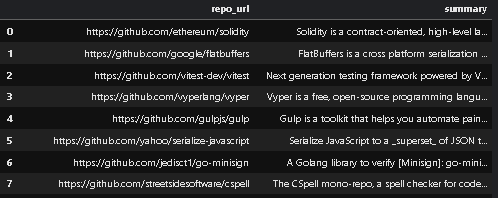
The challenge involves predicting funding allocations between pairs of open-source software repositories. The data provided includes:
- Repositories: A list of open-source software repositories with various attributes.
- Pairwise Comparisons: Data indicating which repository received more funding in pairwise comparisons.
- Dependency Graph: Information about dependencies between repositories.
Solution Approach
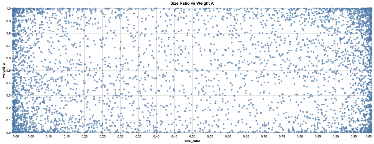
1. Pairwise Comparison Model Using the Bradley-Terry Framework
We implemented a probabilistic Bradley-Terry model to handle pairwise comparisons between repositories. This model is ideal for ranking and predicting outcomes based on pairwise data.
Repository Strength Parameters ((\beta_i)):
Each repository is assigned a parameter representing its “strength” or propensity to receive funding.
Probability Calculation:
The probability that repository i receives funding over repository j is calculated as:
[
P(i \text{ receives funding over } j) = \frac{\beta_i}{\beta_i + \beta_j}
]
Log-Transformation for Optimization:
To facilitate optimization and improve numerical stability, we use the logarithm of the strength parameters:
[
\theta_i = \log(\beta_i)
]
Substituting into the probability equation, we obtain:
[
P(i \text{ receives funding over } j) = \frac{1}{1 + e^{-(\theta_i - \theta_j)}}
]
2. Optimization with the CMA-ES Algorithm
To estimate the parameters ((\theta_i)), we employed the Covariance Matrix Adaptation Evolution Strategy (CMA-ES) optimizer, which is effective for non-linear, non-convex optimization problems.
Objective Function:
We minimize the Mean Squared Error (MSE) between the observed probabilities in the training data and the model’s predicted probabilities:
[
\text{MSE} = \frac{1}{N} \sum_{k=1}^{N} \left( P_{\text{model}}(k) - P_{\text{observed}}(k) \right)^2
]
Regularization:
To prevent overfitting and improve generalization, an L2 regularization term is added:
[
\text{Regularization} = \lambda \sum_{i} \theta_i^2
]
Total Objective Function:
Combining the MSE and the regularization term gives:
[
\text{Objective} = \text{MSE} + \text{Regularization}
]
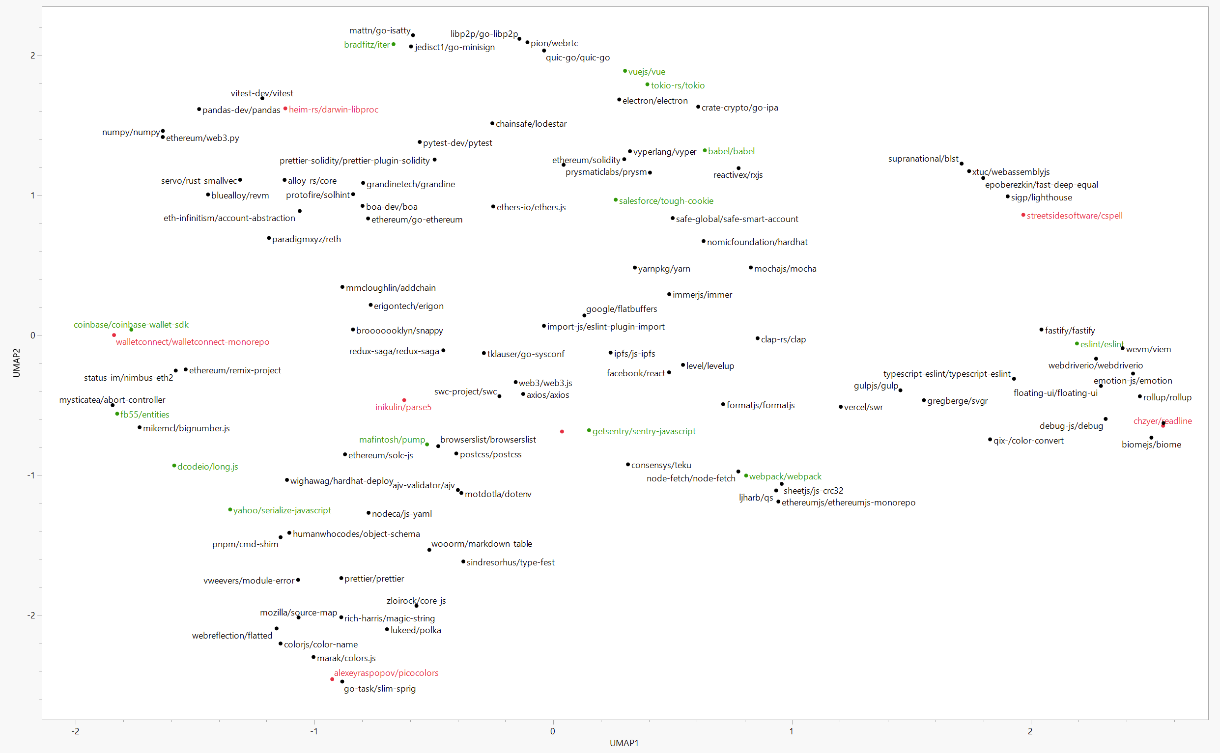
3. Incorporating the Dependency Graph
The dependency graph is integrated into the model to further enhance predictions.
Penalty Terms for Dependencies:
For each edge in the dependency graph, a penalty is added to the objective function based on the difference in (\theta) values of the source (i) and target (j) repositories:
[
\text{Penalty}_{\text{edge}} = \left( (\theta_j - \theta_i) - \log(\text{edge_weight} + \varepsilon) \right)^2
]
Here, (\varepsilon) is a small constant introduced to avoid taking the logarithm of zero.
Default Edge Weights:
For edges without specified weights, a meaningful default value is assigned so that all dependencies contribute to the model.
4. Hyperparameter Tuning and Model Refinement
Hyperparameters are carefully tuned to optimize model performance.
-
Regularization Parameter ((\lambda)):
Values such as (1 \times 10^{-6}) and (1 \times 10^{-5}) were experimented with to balance overfitting and underfitting. The optimal value was chosen based on the validation MSE.
-
Optimizer Settings:
- Max Evaluations: Adjusted to ensure convergence without unnecessary computation.
- Population Size: Determined based on the number of repositories to enhance optimizer performance.
- Sigma Values: Initialized relative to the (\theta) values to effectively guide the optimization process.
-
Validation:
MSE is monitored on a validation set and cross-validation techniques are used to assess model generalization.
5. Prediction and Output Generation
Computing Strength Parameters:
After optimization, the strength parameters for each repository are calculated as follows:
[
\beta_i = e^{\theta_i}
]
Making Predictions:
For each pair in the test data, the prediction is made as follows:
[
P(\text{project_a receives funding over project_b}) = \frac{\beta_{\text{project_a}}}{\beta_{\text{project_a}} + \beta_{\text{project_b}}}
]
Output:
An output is generated that contains the predicted probabilities, ensuring compatibility and facilitating ease of analysis.
Innovations and Advantages of the Solution
Advanced Machine Learning Techniques
-
Probabilistic Modeling:
The use of the Bradley-Terry model captures complex funding allocation dynamics.
-
Effective Optimization:
The CMA-ES optimizer enables efficient optimization in challenging, high-dimensional spaces.
Integration of the Dependency Graph
-
Enhanced Accuracy:
By considering repository dependencies, the model better reflects real-world funding influences.
-
Structural Awareness:
The model accounts for key dependencies, potentially highlighting foundational projects.
Future-Ready with Real-Time Data Integration
-
Airbyte Integration Plans:
Real-time data ingestion from various sources will be used to constantly update repository metrics.
-
Continuous Improvement:
Incorporating the latest trends ensures that the model remains current and adaptive.